

In this tutorial, we will see steps to create simple PivotTable and PivotChart using Excel.
What is a PivotTable?
A PivotTable is a powerful tool to calculate, summarize, and analyze data that lets you see comparisons, patterns, and trends in your data. The trends and comparisons help you to make decisions. Pivot table in its basic form takes data and summarizes it so you can make sense of the data, all without using any formulas!
PivotChart, is a more visual way to summarize and make sense of the data.
Steps to Create a PivotTable
The first step to making a good PivotTable is to make sure the data is in good shape. So, make sure you do the following before you make PivotTable.
Select the cells you want to create a PivotTable from. Your data shouldn’t have any empty rows or columns.
Select Insert > PivotTable.
Choose the data that you want to analyze, select Select a table or range.
To add a field to your PivotTable, select the field name checkbox in the PivotTables Fields pane.
Choose where you want the PivotTable report to be placed, select New worksheet or Existing worksheet and then select the location you want the PivotTable to appear.
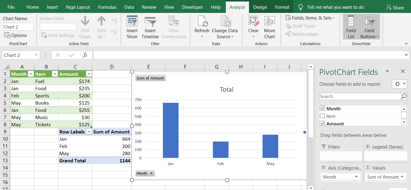

I have created a sample data and generated the PivotTable and chart using the steps above as shown in the screenshot.
PivotTable is not as hard as you think. After you go through simple steps, you’ll know how to quickly create one for your data.